“Last time, I asked: ‘What does mathematics mean to you?’, and some people answered: ‘The manipulation of numbers, the manipulation of structures.’ And if I had asked what music means to you, would you have answered: ‘The manipulation of notes?’” — Serge Lang
Abstractness is the price of generality. — 普适的代价是抽象
定义
$span:$ The “span” of $\vec v$ and $\vec w$ is the set of all their linear combinations.(给定向量张成的空间)
$linearly$ $dependent:$ 一组向量中至少有一个向量对张成的空间大小没有贡献。
$basis:$ The basis of a vector space is a set of linearly independent vectors that span the full space.(向量空间的一组基是张成该空间的一个线性无关向量集)
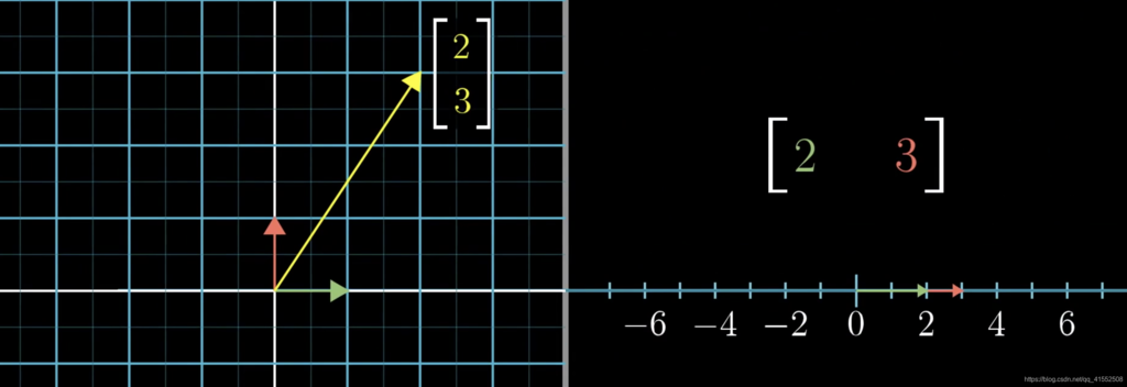
$linear$ $transformation:$ (1) Lines remain lines(直线依旧是直线)(2) Origin remains fixed(原点保持固定)(3) keeping grid lines parallel and evenly spaced(保持网格线平行且等距分布)(4) 线性变换仅对基底进行改变,即 $\vec v=(x,y)=x\cdot \vec i+y\cdot\vec j$ 在线性变换后为 $\vec v’=x\cdot \vec i’+y\cdot\vec j’$
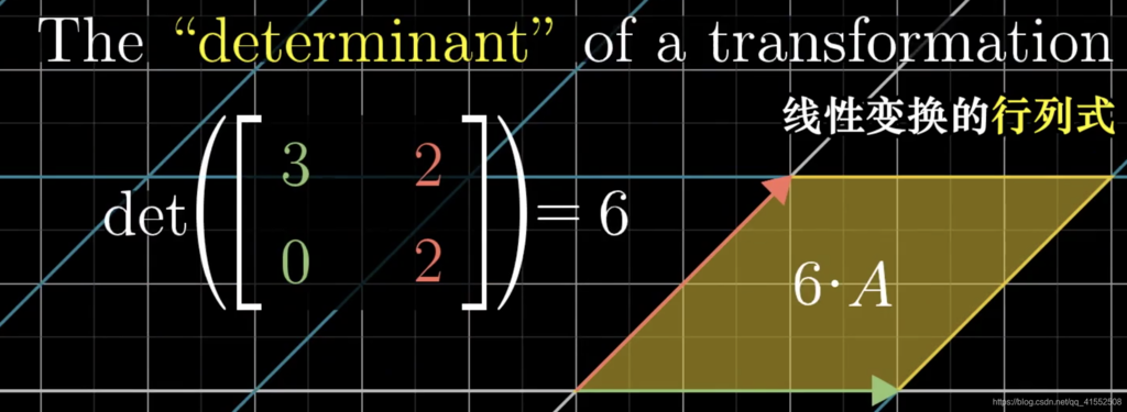
$determinant:$ 矩阵行列式,即线性变换改变面积的比例。
-
若 $det(A)=0$,则整个平面被压缩到一条线甚至一个点上 ,即空间被压缩到了更小的维度上。
-
若 $det(A)<0$,则空间定向发生了改变,例如二维平面上 $\vec i$ 出现在 $\vec j$ 的左边。(the orientation of space has been inverted)
-
$det(M_1M_2)=det(M_1)det(M_2)$
$rank:$ Number of dimensions in the output.(秩,矩阵列空间的维数)
$column$ $space:$ Set of all possible outputs $A\vec v$.($A$ 的列空间,即矩阵的列所张成的空间)
$null$ $space$ / $kernel:$ The set of vectors that lands on the origin is called the “null space” or the “kernel” of the matrix.(变换后落在原点的向量的集合,被称为矩阵的 “零空间” 或 “核”;变换后一些向量落在零向量上,而 “零空间” 正是这些向量所构成的空间)
-
举例,$null$ $space$ $of$ $A=\{x\mid Ax=0\}$
- 另外,零空间的维度等于列数减去秩
$duality:$ Natural-but-surprising correspondence between two types of mathematical thing.(对偶性,自然而又出乎意料的对应关系)
- 一个向量的对偶是由它定义的线性变换
- 一个多维空间到一维空间的线性变换的对偶是多维空间中的某个特定向量
$eigenvector:$ 线性变换后仍位于原直线上的向量
$eigenvalue:$ 特征向量的放缩倍数,如果为负数,则方向相反
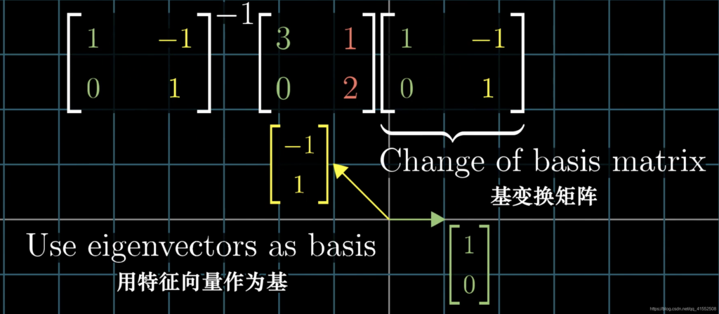
$eigenbasis:$ 特征基,由特征向量组成的基,可用于矩阵特征值分解(例如可以加速矩阵幂次运算)
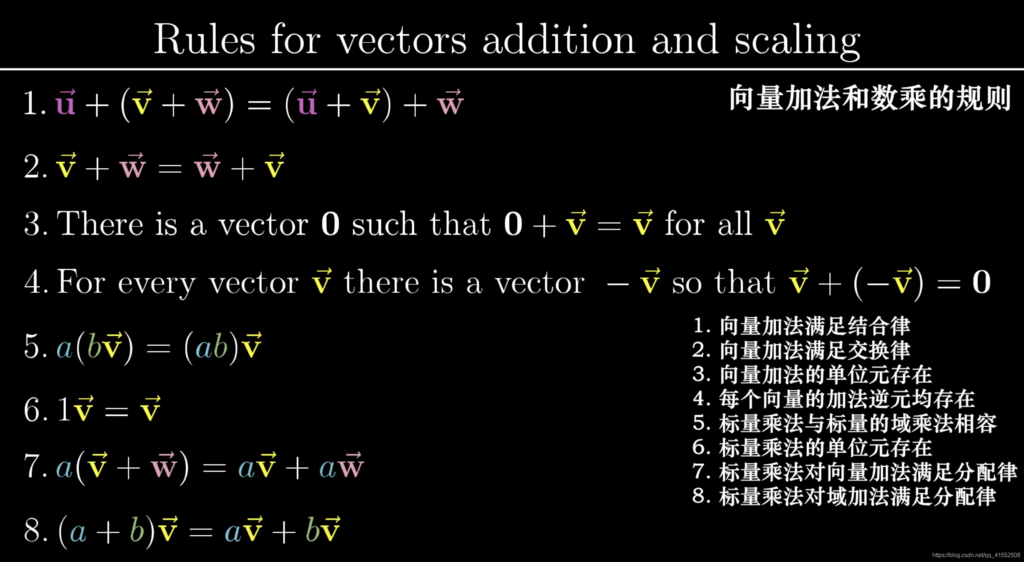
$vector$ $spaces:$ 箭头、一组数、函数等类似向量的事物,它们构成的集合被称为 “向量空间”。(满足下述八条公理 - Axioms 即为向量)
$orthogonal$ $transformation:$ If $T(\vec v)\cdot T(\vec w)=\vec v\cdot \vec w$ for all $\vec v$ and $\vec w$, $T$ is “Orthonormal”.(基底仍为单位向量且互相垂直,向量变换后长度不变)
性质
-
Linear algebra revolves around vector addition and scalar multiplication.(线性代数紧紧围绕向量加法与数乘)
-
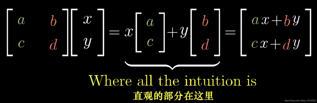
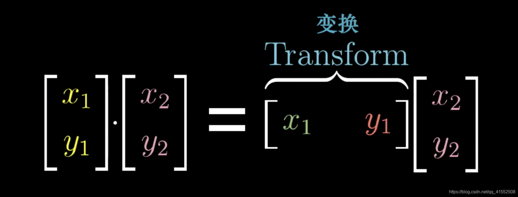
[矩阵] [向量]:对向量做线性变换,本质是更换向量所在空间的基底,其中矩阵的第 $i$ 列对应更换后的第 $i$ 维基底。
-
[矩阵] [矩阵]:apply one transformation after another, (1) $AB\not=BA$, (2) $ABC=A(BC)$
-
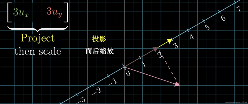
[向量] $\cdot$ [向量]:两个向量点乘,就是将其中一个转化为线性变换
-
线性变换 $L$ 的严格定义:(1) $L(\vec v+\vec w)=L(\vec v)+L(\vec w)$, (2) $L(c\vec v)=cL(\vec v)$
-
基向量的变换
-
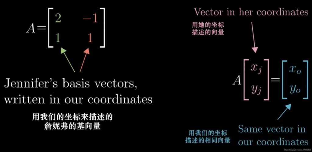
$A^{-1}MA:$ 暗示着一种数学上的转移作用,即先用 $A$ 将坐标系线性变化(更换基),再执行 $M$(直观的线性变换),再回归到原来的坐标系($A^{-1}$)。
-
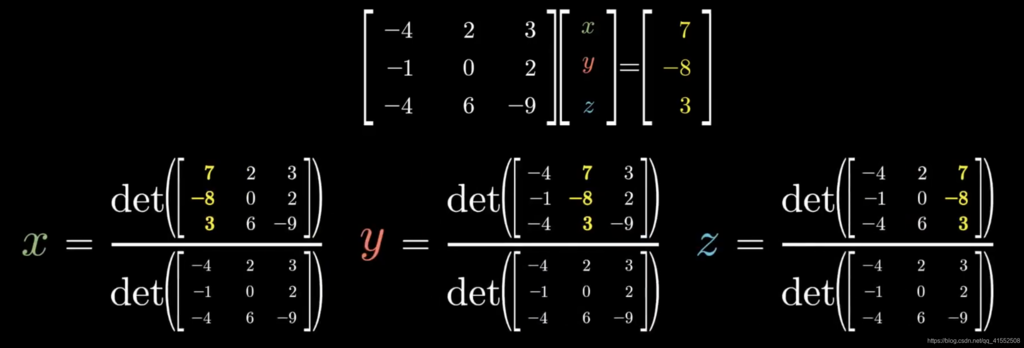
克莱姆法则:根据行列式代表空间变换大小的性质,求解每一个未知量时,固定其它维度的基不变,仅改变当前基,使得变换后空间大小恒等。
其它
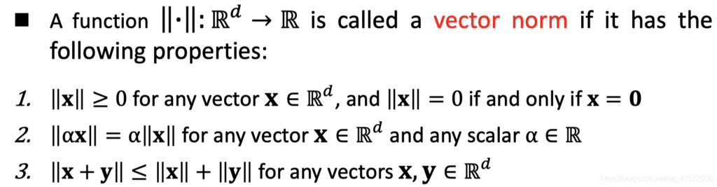
向量范数 (Vector Norms)
-
$x\in \mathbb{R}^d$
-
$l_p\text{-}norm=||x||_p=(\sum\limits_{i=1}^d|x_i|^p)^{1/p}$
-
$l_2\text{-}norm=Euclidean\ norm$
-
$l_0\text{-}norm=||x||_0=\sum_{i=1}^dI(x_i>0)$
-
$l_{\infty}\text{-}norm=||x||_{\infty}=\underset{1\leq i\leq d}{\max}|x_i|$
矩阵范数 (Matrix Norms)
-
$A\in \mathbb{R}^{m\ \text{x}\ n}$
-
$||A||_2=\sigma_1$,即最大的奇异值
-
$||A||_{Nuclear}=\sum\limits_{i=1}^r\sigma_i$
-
$||A||_p=||vec(A)||_p=(\sum\limits_{i=1}^m\sum\limits_{j=1}^n|x_{ij}|^p)^{1/p}$
-
$||A||_{p,q}=(\sum\limits_{i=1}^m(\sum\limits_{j=1}^n|a_{ij}|^p)^{q/p})^{1/q}$
-
Frobenius norm $=||A||_{2,1}=||A||_F=(tr(A^TA))^{1/2}=(\sum\limits_{i=1}^m\sum\limits_{j=1}^na_{ij}^2)^{1/2}$
矩阵的迹
-
For a square matrix $A$
-
Trace: sum of diagonal elements, $tr(A)=\sum\limits_{k=1}^da_{kk}$
-
$tr(A)=tr(A^T)$
-
$tr(\alpha A+\beta B)=\alpha tr(A)+\beta tr(B)$
-
$tr(ABC)=tr(BCA)=tr(CAB)$
-
$tr(A^TB)=\sum_{i=1}^n\sum_{j=1}^ma_{ij}b_{ij}=<A,B>$
特征值
-
$A\in \mathbb{R}^{m\ \text{x}\ m}$
-
$Av=\lambda v$, $v$ is an eigenvector, $\lambda$ is the corresponding eigenvalue.
-
$tr(A)=\sum_i\lambda_i$
-
$det(A)=|A|=\prod_i\lambda_i$
- 幂法求矩阵特征值
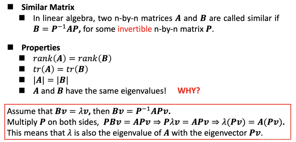
相似矩阵 (Similar Matrix)
常见转换
-
$\left(A+B D^{-1} C\right)^{-1}=A^{-1}-A^{-1} B\left(D+C A^{-1} B\right)^{-1} C A^{-1}$
-
$\det(I_{N}+A B^{\top})=\det(I_{M}+A^{\top} B)$ 当矩阵 $A,B$ 均为 $m\cdot n$ 时成立
矩阵 / 向量求导
-
分子布局:分子按列展开
-
分母布局:分母按列展开(通常采用)
-
$x:$ 标量,$\textbf{x}:$ 向量,$A:$ 矩阵
-
$\displaystyle\frac{d}{d\textbf{x}}(A\textbf{x})=A^T$
-
$\displaystyle\frac{d\textbf{x}}{d\textbf{x}}=I$
-
$\displaystyle\frac{d\textbf{y}^T\textbf{x}}{d\textbf{x}}=\displaystyle\frac{d\textbf{x}^T\textbf{y}}{d\textbf{x}}=\textbf{y}$
-
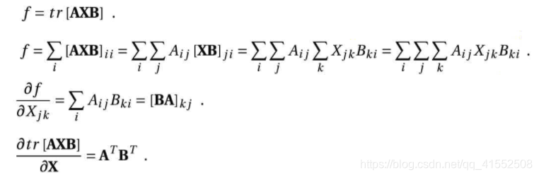
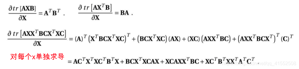
$\displaystyle\frac{\partial \mathbf{a}^{T} \mathbf{X} \mathbf{b}}{\partial \mathbf{X}}=\mathbf{a b}^{T}$
-
$\displaystyle\frac{\partial \mathbf{a}^{T} \mathbf{X}^{T} \mathbf{b}}{\partial \mathbf{X}}=\mathbf{b a}^{T}$
-
$\displaystyle\frac{d}{d\textbf{x}}(\textbf{x}^TA\textbf{x})=(A+A^T)\textbf{x},\textbf{x}^TA\textbf{x}=\sum\limits_{i=1}^n\sum\limits_{j=1}^nx_ix_jA_{ij}$
-
$\displaystyle\frac{d}{d\textbf{W}}(p^{T} \textbf{W} t)=\displaystyle\frac{d}{d\textbf{W}}(t^{T} \textbf{W}^T p)=pt^{T}$
-
$\displaystyle\frac{d}{d\textbf{X}}(\log\det\mathbf{X})=\mathbf{X}^{-1},\mathbf{X}\in\mathbf{S}^n_{++}$
-
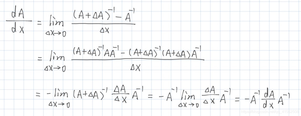
$\displaystyle\frac{d \mathbf{A}^{-1}}{d x}=-\mathbf{A}^{-1} \frac{d \mathbf{A}}{d x} \mathbf{A}^{-1}$
- $Trace$